What Are Logistics Feedback Loops, and Why Should You Care about Them?

The role of feedback loops in logistics processes receives relatively scant attention; however, these tools play an essential role in logistics planning and execution. Specifically, feedback loops act to assure alignment between plans developed at the strategic, tactical and operational levels, and to facilitate efficient, coordinated operational execution. While feedback loops represent a relatively underpublicized topic, the functionality they provide is critical in practice.
What is a Feedback Loop?
The conceptual basis for feedback loops is that planning decisions made at higher levels (e.g., the 12-18 month tactical planning level) are sometimes infeasible or flawed when implemented at lower levels. To minimize a company’s vulnerability to this planning danger, it is important to design mechanisms that incorporate (or feedback) information from lower level planning horizons (e.g., the short term operational) to higher levels (e.g., the 12-18 month tactical planning level).
To illustrate a tangible example of a feedback loop, let’s briefly consider the hierarchical manufacturing and distribution (HMD) planning framework displayed in Figure 1.
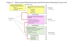
A distinguishing characteristic of a hierarchical logistics planning framework is that decisions made at higher planning levels (e.g., the strategic level) place constraints and boundaries on subsequent decisions that will later be made at lower planning levels (e.g., the tactical level). This facilitates aligned decision making across all levels of a logistics organization and its individual functions from a “top down” perspective.
To strengthen the alignment of organizational decision making, “hierarchical” planning frameworks also employ “feedback loops.” Briefly, feedback loops represent both formal and informal mechanisms by which planners at lower levels of the planning hierarchy provide feedback to planners at higher levels. In Figure 1, the arrows flowing upwards from the operational level to the tactical level, and from the tactical level to the strategic level, represent feedback loops.
Thus, a true HMD framework is a closed loop system which employs a “top down” planning approach complemented by “bottom up” feedback loops. Given the emphasis of HMD systems on evaluating capacity levels, and on imposing and/or communicating capacity constraints from higher levels down to lower levels, it is imperative that strong feedback loops exist. Without proper feedback loops imbedded into a hierarchical planning framework, the danger that a logistics function will attempt to move forward with infeasible plans always exists. These infeasibilities often do not surface until an organization is in the midst of executing its operational plans and schedules.
Feedback loops take many forms and can range from: (1) informal communications between two logistics functions, to (2) formal, standardized data input and output exchanges between functions; to (3) detailed mathematical algorithms that coordinate modeling assumptions and inputs between different planning and operating levels. This example will illustrate the need for a manufacturer to evaluate its inventory at the end item level across its entire network, in order to determine the correct product family beginning inventory level inputs to its annual/tactical production planning process. Thus, the following is an example of a feedback loop required to assure synchronization between current manufacturing/distribution inventory network operating conditions and annual/tactical production planning. (This feedback loop thus facilitates inventory data analysis, development and exchange between the operational and tactical planning levels.)
Manufacturing and distribution firms with thousands of unique finished goods end items typically develop their annual or tactical production and distribution plans at an aggregated product level. Numerous reasons exist for this planning approach, not the least of which is that it is often simply not practical or productive to develop long run plans (e.g., 12-18 months) for thousands of individual end items.
Product Line Structure
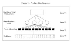
Figure 2 illustrates the levels of product aggregation which we assume. One can observe that end items tree up into product families, and product families then tree up into product lines. The example here assumes that the firm’s annual production/distribution planning model defines products at the product family level (level 3 in Figure 2). Product families are created based upon the similarity of one or more key commonly shared characteristics of each end item within a family. (In the production planning application for which the authors developed and implemented the analytic example described here, all end items within each family had virtually identical production rates, costs and production possibilities.)
Why Is It Critical to Incorporate End Item Inventory Positions into Annual Product Family Level Production Plans?
It is necessary to evaluate current end item inventory positions over the entire manufacturing/distribution network in order to assure that the firm’s annual production plans do not underestimate total manufacturing capacity requirements. Inventory data, when developed at the product family level (rather than at the end item level), can provide misleading information leading to this underestimation of capacity requirements in long run planning models.
To illustrate this, assume we are planning the annual production requirements of a product family that has five individual end items. Let us now consider the production requirements over a planning horizon for this product family when evaluated at two different levels of inventory aggregation: the end item level, and the product family level. To measure the utility of a product family’s current inventory, we require two definitions. (Note: “Useable” inventory is the amount of beginning inventory that can be used to meet forecast sales and the end of planning horizon inventory target. “Excess” inventory is the amount of beginning inventory (if any) that is not needed to meet the forecast sales and end of planning horizon inventory target.)
“Useable” inventory over the planning horizon is the maximum of:
(forecast annual sales over the planning horizon) + (the end-of-period inventory target) – (the current, i.e., beginning-of-period inventory), or 0.
“Excess” inventory over the planning horizon is the maximum of:
(current or beginning-of-period inventory) – (useable inventory over the planning horizon), or 0.
A comparison of Figures 3 and 4 reveals that the projected total production requirements over the planning horizon can vary substantially depending upon whether one evaluates requirements at the end item level (Figure 3, column 5 – “11,000”), or at the product family level (Figure 4, column 4 – “8,000”). Specifically, the firm risks underestimating its true production capacity requirements if it evaluates inventory at the product family level.
In this example, column 7 of Figure 3 illustrates that the underestimate of capacity needs will occur because end item 5 has an extreme surplus of inventory which masks the current inventory deficits in items 1 through 4 of this family. Because item 5’s current inventory exceeds the sum of its annual selling rate plus inventory target by 3,000 units, the firm will still have an inventory excess of 3,000 units in this item at the end of its twelve-month planning horizon. To plan production requirements accurately, the firm must recognize that it has 3,000 units of inventory in item 5 (and therefore in item 5’s product family) that it cannot utilize over the planning horizon. For production planning purposes, including these 3,000 units in the product family’s current inventory figure will overstate the true level of inventory “useable over the planning horizon” for this product family. Thus, the number displayed in column (6) of Figure 3 (8,000) rather than the number in column (5) of Figure 4 (11,000) represents the proper quantity to use as this family’s “beginning-of-period inventory” in an annual production/distribution planning model. Further, the firm will need to plan on production of 11,000 units of this product family in its annual plan rather than just 8,000 units.
Obviously for other reasons (e.g., financial, marketing excess inventory disposal promotions, etc.), one must account for this product family’s excess inventory (over the planning horizon) in other planning areas.

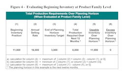
The example in Figure 4 illustrates that evaluating inventory positions (and production requirements) at the product family level makes it impossible to recognize if there is any excess or unusable inventory (over the planning horizon) in any of the end items within the product family. By using the approach shown in Figure 3, namely, evaluating inventory positions and production requirements at the end item level, and then summing the end item results to obtain product family requirements, one can accurately evaluate a product family’s current level of “useable” inventory over the planning horizon.
Determining Useable and Excess Inventory over a Planning Horizon for a Multi-location Network
The example in Figure 3 demonstrates the calculation of useable and excess inventory over the planning horizon for a stand-alone, one location manufacturing/distribution network. In the real world of multi-location networks, the determination of proper useable and excess inventory data for product families becomes more complex. However, the same basic logic used for the one location network can easily be extended to a multi-location, multi-echelon network.
This section has presented a simple yet effective method for developing beginning-of-period inventory data at the product family level for use in tactical production/distribution planning models. Developing beginning-of-period product family inventory data using the approach described here creates the necessary link (i.e., feedback loop) between long run production/distribution planning and short run, current inventory conditions.
Summary
Our example demonstrated that input from the operational level back up to the tactical planning level (i.e., a feedback mechanism) was required to identify the correct inventory data for long run production planning. More generally, feedback loops from lower planning and operational levels to higher levels take many forms and cover numerous activities. What is key is that a firm build as many feedback loops into its standard business processes as required. This safeguards that plans created at higher, more aggregated planning horizons are thoroughly vetted at lower operating levels to identify any key bottlenecks or potential issues previously undetected. Further, an organization that actively imbeds feedback loops into its business processes fosters an open and transparent environment in which short run issues encountered at operational levels, or medium term issues encountered at tactical levels, are promptly communicated back to the appropriate planning levels above them for analysis and redressing.
Additional Perspective
Another brief example of feedback loops illustrates that these mechanisms can be both formal and analytically-based, such as the inventory planning example just presented in this article, or alternatively can be more informal and qualitative in nature. Figure 5 outlines an illustration of a loose (“informal”) feedback system that a ceramic tile firm implemented.
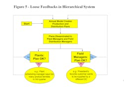
Briefly, the firm utilized mathematical optimization models to generate integrated annual production and distribution plans for all its plants and distribution centers. A key element of this rigorous planning process, however, consisted of the more informal feedback system depicted in Figure 5 where all key field personnel were required to provide their assessments of a plan once it was developed. These assessments were collected and if warranted, tactical plans initially developed at headquarters would be recalibrated taking these assessments (feedbacks) into consideration. As Figure 5 depicts, the feedback provided was often a mix of non-analytic and analytic considerations.
Tan Miller is director of the Global Supply Chain Management Program at Rider University’s Norm Brodsky College of Business, and a member of MH&L’s Editorial Advisory Board.
Matthew J. Liberatore, PhD, is John F. Connelly Chair in Management, Villanova School of Business, Villanova University.